The Phillips Curve & the Aggregate Supply
Week 07
March 23, 2026
The Pains of Fighting Inflation
“We have got to get inflation behind us. I wish there were a painless way to do that.” There isn’t.” Jerome Powell, Fed’s Chair, 21 Sept. 2022

The Pains of Fighting Inflation
“We have got to get inflation behind us. I wish there were a painless way to do that.” There isn’t.” Jerome Powell, Fed’s Chair, 21 Sept. 2022
The Phillips Curve (PC)
- Alban Phillips discovered in the 1950s the kind of pain we have to suffer from reducing inflation.
- The PC shows how much more unemployment we will get \((\uparrow U)\), to reduce the inflation rate \((\downarrow \pi)\).
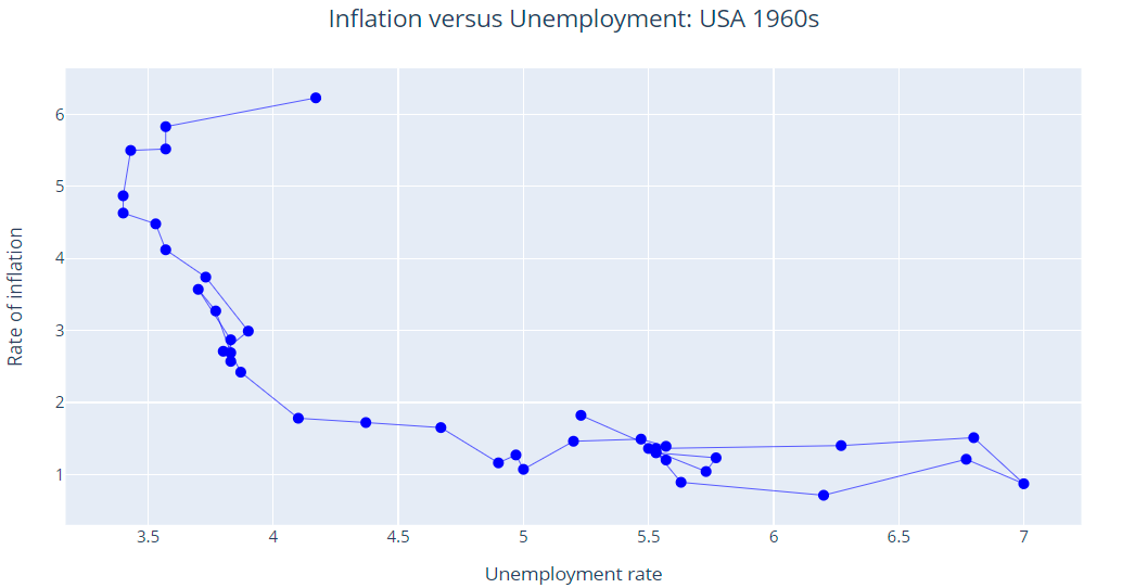
- The PC was easily confirmed in the 1960s.
- See next figure (click on any key)
![]() .
.
The Phillips Curve (PC)
In the 1960s, the PC was easy to spot and confirmed Phillips discovery.
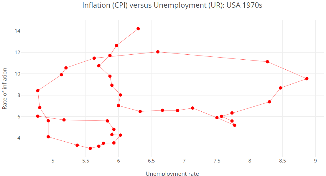
The Phillips Curve in the 1970s
- In the 1970s, the PC begins to display a strange configuration: it seems to move constantly, looping around.
\(~~~~~\)
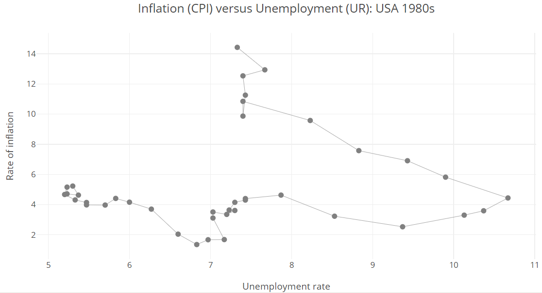
The Phillips Curve in the 1980s
- In the 1980s, the PC seems to have different slopes.
\(~~~~~\)
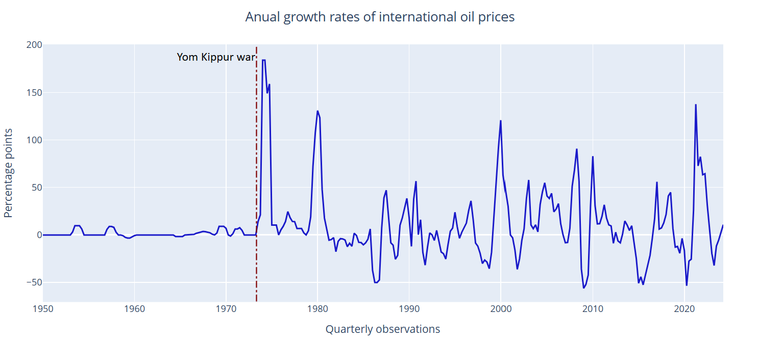
Oil Price Shocks
Large shocks in oil prices have been a recurrent major characteristic of the world economy since the early 1970s. They are temporary shocks.
The PC: Graphical Representation
\[\pi=\pi^e-\omega\left(U-U^n\right)+\rho \quad , \quad \color{black}{\pi^e=\pi_{-1}}\]
- If we want a lower unemployment rate \((\downarrow U)\)
- We have to accept a higher inflation rate \((\uparrow \pi)\)
- Assuming everything else constant \(\left(U^n, \pi^e, \rho\right)\).
- Graphically, this can be represented as in the next figure (click on any key)
![]()
The PC: Graphical Representation
\[\pi=\pi^e-\omega\left(U-U^n\right)+\rho \quad , \quad \color{black}{\pi^e=\pi_{-1}}\]
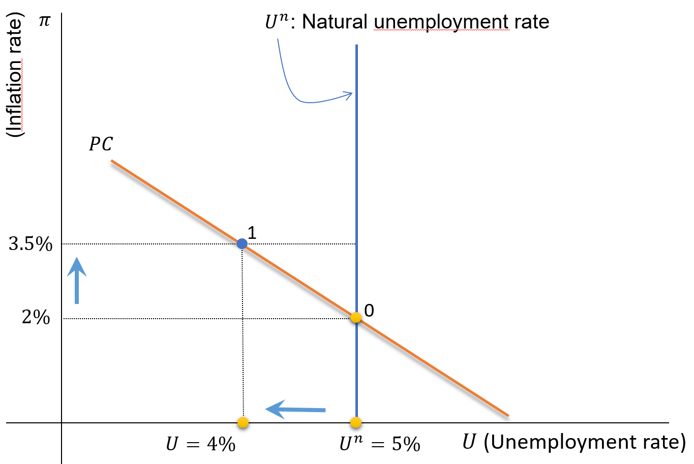
Example:
- \(\pi_{-1} = 2\%\),
- \(\omega=1.5\)
- \(U^n=5\%\)
- If \(U=4\%\)
- \(U<U^n \Rightarrow \uparrow \pi\)
- \(\pi=3.5\%\)
Shifts in the Phillips Curve \((\pi^e , \ \rho)\)
\[\pi=\pi^e-\omega\left(U-U^n\right)+\rho \quad , \quad \color{black}{\pi^e=\pi_{-1}}\]
- The Phillips Curve shifts when the following forces change:
- Expected inflation (\(\pi^e\))
- Supply shocks (\(\rho\))
- Natural unemployment rate (\(U^n\))
- Let us concentrate on the first two forces (click on any key).
![]()
Shifts in the Phillips Curve \((\pi^e , \ \rho)\)
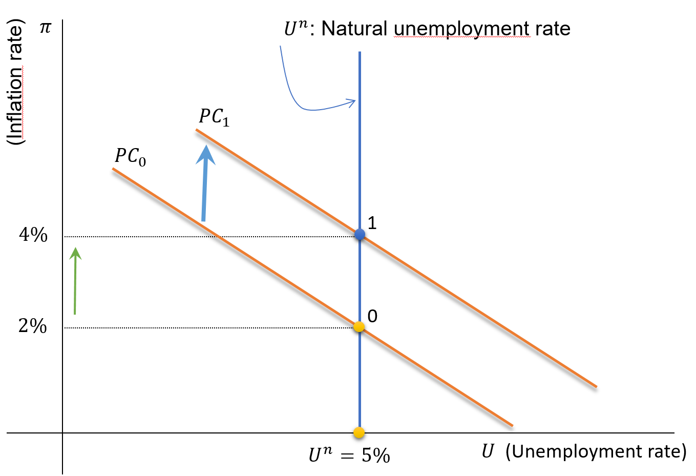
The PC shifts to the right if:
- \(\uparrow \pi^e\), \(~~\) or
- \(\uparrow \rho\)
Shifts in the Phillips Curve (\(U^n\))
\[\pi=\pi^e-\omega\left(U-U^n\right)+\rho \quad , \quad \color{black}{\pi^e=\pi_{-1}}\]
- The Phillips Curve shifts when the following forces change:
- Expected inflation (\(\pi^e\))
- Supply shocks (\(\rho\))
- Natural unemployment rate (\(U^n\))
- Let us concentrate on the last force (click on any key).
![]()
Shifts in the Phillips Curve (\(U^n\))
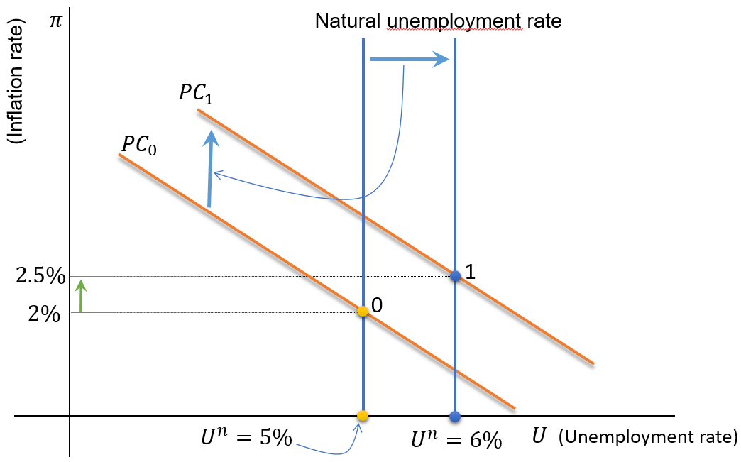
The PC will shift to the right if:
- \(\uparrow U^n\)
- Stable inflation will now be at 2.5%
Shifts in the PC: Inflationary Spiral Numerically
\[\pi=\pi^e-\omega\left(U-U^n\right)+\rho \quad , \quad \color{black}{\pi^e=\pi_{-1}}\]
- What happens if the government or the central bank try to keep the unemployment rate below the natural rate ?
- \(U<U^n\)
- The Phillips Curve will shift to the right
- \(U<U^n\)
- Inflationary expectations : inflation will increase systematically over time
![]()
Shifts in the PC: Inflationary Spiral Numerically
\[\pi=\pi^e-\omega\left(U-U^n\right), \quad \omega=1.5, \quad \pi_t^e=\pi_{t-1}\]
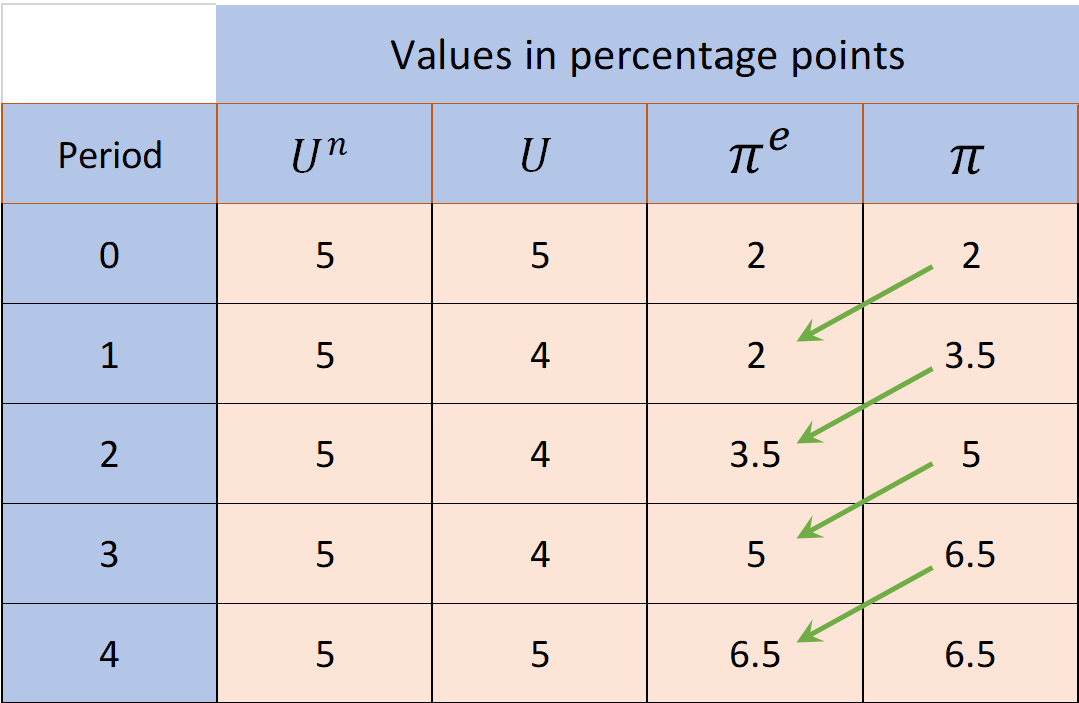
- Suppose \(\pi _0 =2\%\)
- If, \(U_1<U^n_1\) Inflation will only stop if \(U\) returns to the \(U^n\) level
- But the result will be a higher \(\pi\) and the same initial \(U\)
Shifts in the PC: Inflationary Spiral Graphically
\[\pi=\pi^e-\omega\left(U-U^n\right), \quad \omega=1.5, \quad \pi_t^e=\pi_{t-1}\]
- The previous numerical example can be represented graphically
- Click on any key to continue
![]()
Shifts in the PC: Inflationary Spiral Graphically
\[\pi=\pi^e-\omega\left(U-U^n\right), \quad \omega=1.5, \quad \pi_t^e=\pi_{t-1}\]
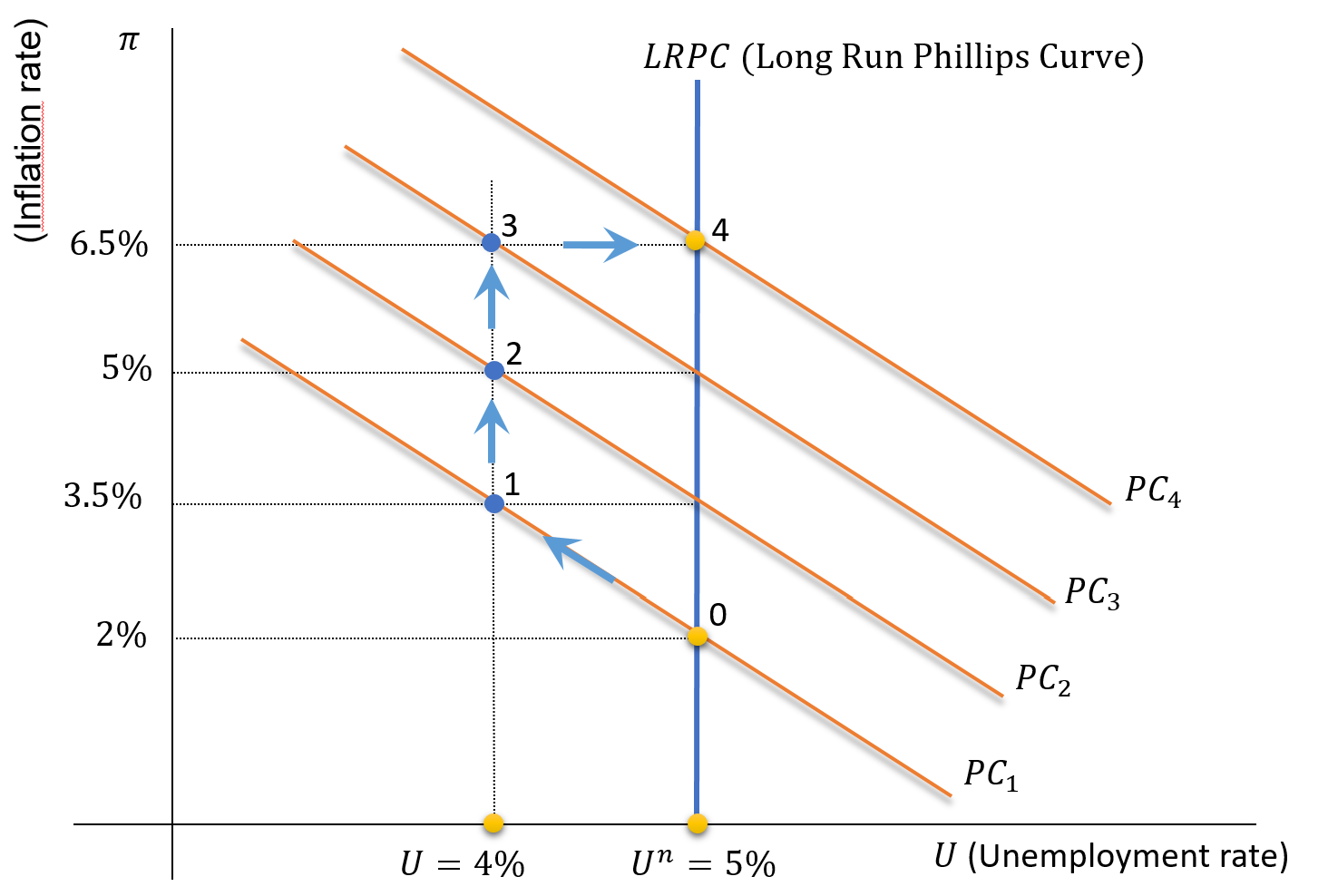
- Suppose \(\pi _0 =2\%\)
- Inflation will only stop if the \(U\) returns to the \(U^n\) level
- But the result will be a higher \(\pi\) and the same initial \(U\)
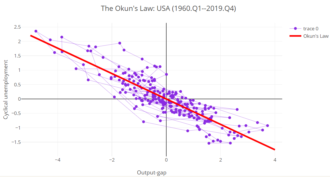
The Okun’s Law for the USA
The slope of the curve was \(−0.441\) for the period 1960-2019.
The AS Curve: Graphical Representation
\[ \pi=\pi^e+\gamma\left(Y-Y^P\right)+\rho \quad , \quad \pi^e = \pi_{-1} \]
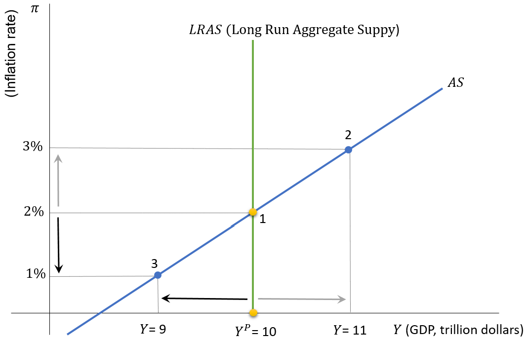
- In 1, \(Y=Y^P\)
- In 2, \(Y>Y^P\), economic boom, \(\pi\) increases to \(3\%\)
- In 3, \(Y<Y^P\), economic recession, \(\pi\) decreases to \(1\%\)
Shifts in the AS Curve (\(\pi^e, \rho\))
\[ \pi=\pi^e+\gamma\left(Y-Y^P\right)+\rho \quad , \quad \pi^e = \pi_{-1} \]
- The AS Curve shifts when the following forces change:
- Expected inflation (\(\pi^e\))
- Supply shocks (\(\rho\))
- Potential GDP (\(Y^P\))
- Let us concentrate on the two first forces (click on any key).
![]()
Shifts in the AS Curve (\(\pi^e, \rho\))
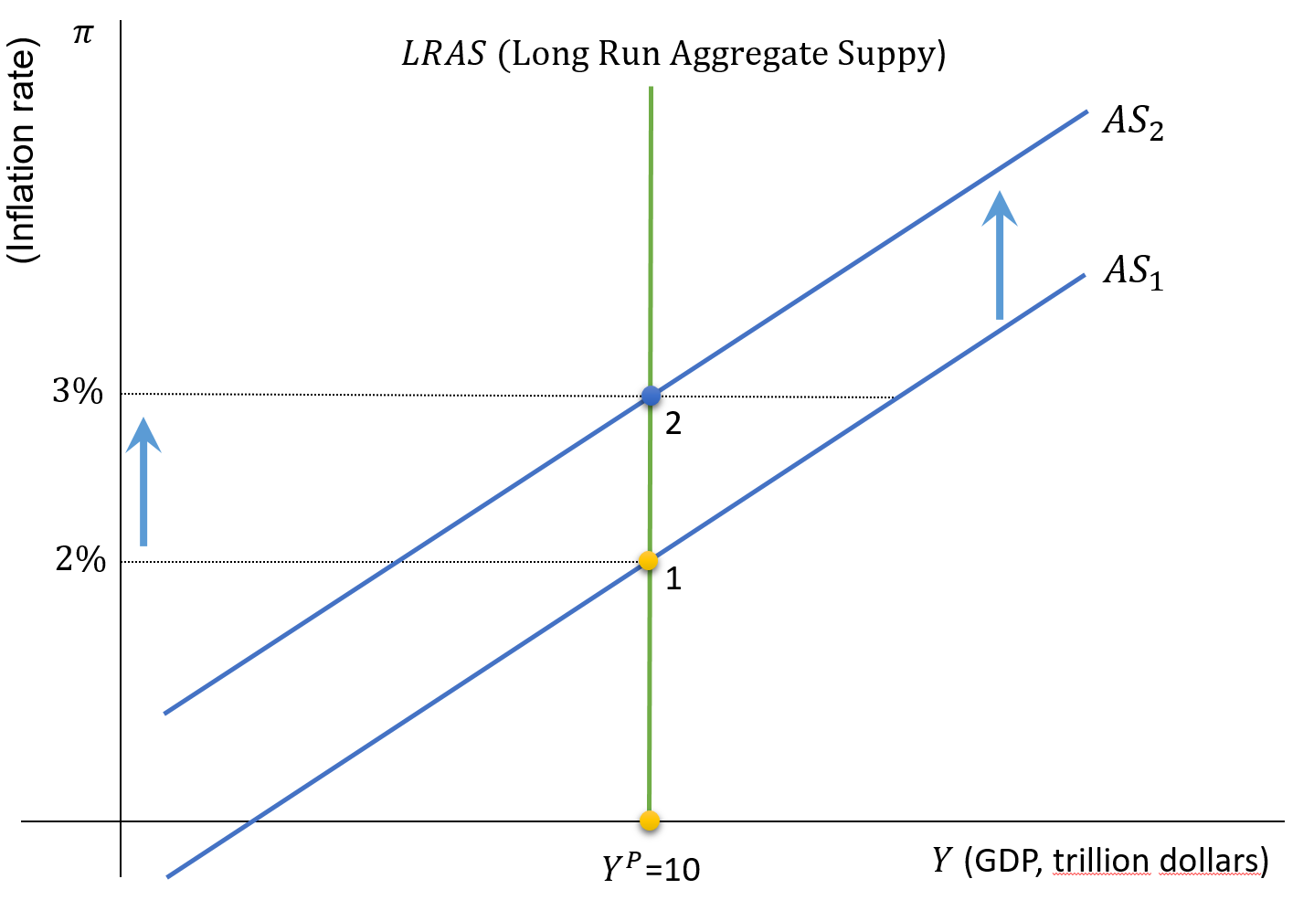
The AS shifts to the left if:
- \(\uparrow \pi^e\), or
- \(\uparrow \rho\)
Shifts in the AS Curve (\(Y^P\))
\[ \pi=\pi^e+\gamma\left(Y-Y^P\right)+\rho \quad , \quad \pi^e = \pi_{-1} \]
- The AS Curve shifts when the following forces change:
- Expected inflation (\(\pi^e\))
- Supply shocks (\(\rho\))]
- Potential GDP (\(Y^P\))
- Let us concentrate on the last force (click on any key).
![]()
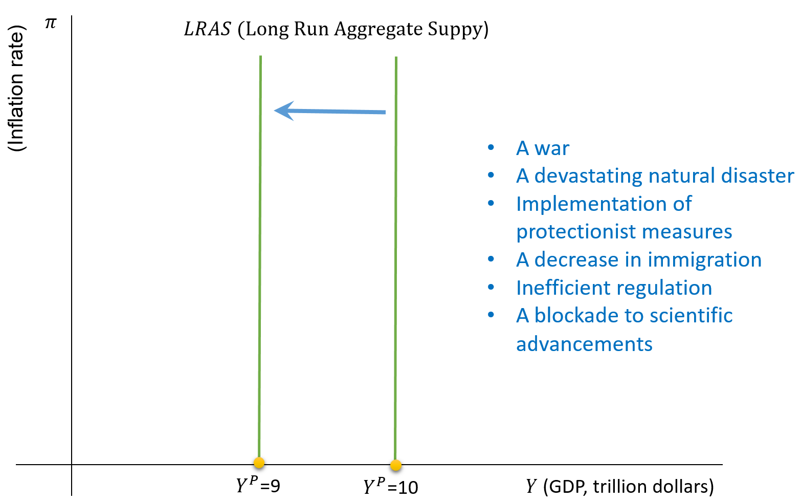
Shifts in the AS Curve (\(Y^P\))
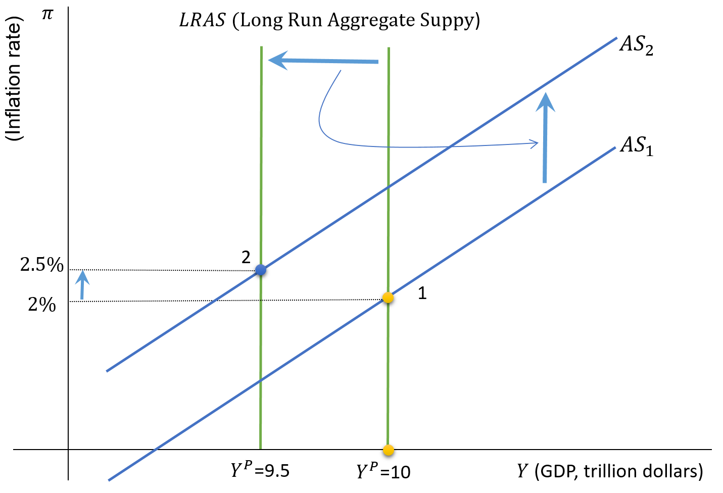
AS shifts to the left if:
- \(\downarrow Y^P\)
- The economy will have stable \(\pi\) only at point 2.
- At 2: \(\ \downarrow Y \ \) , \(\ \uparrow \pi\)
What Factors Shift the LRAS Curve?
Forces reducing any of the factors \(\{\cal{T}, K, L\}\) shift the LRAS to the left, and vice-versa.